Control module¶

This section describes the most important tools of the Control module with examples. For a more detailed description of the methods refer to the API.

The Controller Module contains the following classes:

Model Predictive Control (NMPC)

Nonlinear Model Predictive Control¶

The class NMPC implements the Model Predictive Controller. To setup an MPC properly you need at least to define

A horizon length using the horizon property.
An objective function.

In the next following two paragraphs we give more details on these two mandatory settings.

Prediction and control horizon¶

If you only horizon then Neo will assume that control and prediction horizon are the same. To set a control horizon different than the prediction horizon use prediction_horizon and control_horizon separately for example:

nmpc = NMPC(model)
nmpc.control_horizon = 4
nmpc.prediction_horizon = 10

Objective function¶

Neo offers a flexible way for constructing the objective function. This can be set using any combination of these methods:

quad_stage_cost set a quadratic stage cost of the kind \(\Vert (\cdot) \Vert_W^2\)
quad_terminal_cost set a quadratic terminal cost of the kind \(\Vert (\cdot) \Vert_W^2\)
stage_cost (beta) sets a generic stage cost function \(l(x,u)\)
terminal_cost (beta) set a generic terminal cost function \(e(x,u)\)

The quadratic costs have support for path-following, trajectory following and reference tracking problems. While stage_cost and terminal_cost do not support those problem yet.

The creation of the objective function is very flexible. You can call the quadratic terminal and stage cost multiple times. Note that this will add the cost to the previously defined cost. For example, let us suppose you want to define the following objective function

\[\begin{split}L(x,u) = \int_{0}^{T} ( a(t), c(t) )^T \begin{bmatrix} 10 & 0 \\ 0 & 10 \end{bmatrix} ( a(t), c(t) ) + 5 u(t)^2 + b(T)^2\end{split}\]

where \(x = [a,b,c]\) are the model states. The code could look like this

nmpc = NMPC(model)
nmpc.quad_stage_cost.add_states(names=['a', 'c'],  weights=[10, 10])
nmpc.quad_stage_cost.add_inputs(names=['u'],  weights=5)
nmpc.quad_terminal_cost.add_states(names=['b'],  weights=1)

which is equivalent to

nmpc = NMPC(model)
nmpc.quad_stage_cost.add_states(names=['a'],  weights=10)
nmpc.quad_stage_cost.add_states(names=['b'],  weights=10)
nmpc.quad_stage_cost.add_inputs(names=['u'],  weights=5)
nmpc.quad_terminal_cost.add_states(names=['b'],  weights=1)

note how the state \(b\) is added separately.

Note that if you pass a vector to the weights parameters, HILO-MPC will assume that you want to use a diagonal matrix. You can pass directly a matrix, just make sure that the dimensions are correct! For example the following objective function

\[\begin{split}L(x,u) = \int_{0}^{T} ( a(t), c(t) )^T \begin{bmatrix} 10 & 3 \\ 1 & 10 \end{bmatrix} ( a(t), c(t) )\end{split}\]

can be defined as follows

import numpy as np
nmpc = NMPC(model)
nmpc.quad_stage_cost.add_states(names=['a', 'c'],  weights=np.array([[10,3],[1,10]]))

You can mix up things also, for example you might want a state to follow a path with a path following problem while another tracks a reference:

import casadi as ca

nmpc = NMPC(model)

# Create path variable
theta = nmpc.create_path_variable()

nmpc.quad_stage_cost.add_states(names=['a'], weights=[10],
                                ref=ca.sin(theta), path_following=True)
nmpc.quad_stage_cost.add_states(names=['b'], weights=[10],
                                ref=[1])
nmpc.quad_terminal_cost.add_states(names=['a'], weights=[10],
                                   ref=ca.sin(theta), path_following=True)

Note that in this case the state \(b\) is wanted to a fixed reference equal to \(1\) while \(a\) needs to follow a sinusoidal path using path following MPC.

Things can get even more crazy. You can create a path-following trajectory-tracking and reference tracking in the same MPC:

import casadi as ca

time = nmpc.create_time_variable()
theta = nmpc.create_path_variable()

nmpc.quad_stage_cost.add_states(names=['a'], weights=[10],
                                ref=ca.sin(theta), path_following=True)
nmpc.quad_terminal_cost.add_states(names=['a'], weights=[10],
                                   ref=ca.sin(theta), path_following=True)

nmpc.quad_stage_cost.add_states(names=['b'], weights=[100],
                                ref=ca.sin(2 * time), trajectory_tracking=True)
nmpc.quad_terminal_cost.add_states(names=['b'], weights=[100],
                                   ref=ca.sin(2 * time), trajectory_tracking=True)

nmpc.quad_stage_cost.add_states(names=['c'], weights=[100], ref=1)
nmpc.quad_terminal_cost.add_states(names=['c'], weights=[100], ref=1)

Note how \(a\) wants to follow a path,:math:b a time-varying trajectory and \(c\) a constant reference! You can do that, sure… but if that makes sense for your problem is up to you to decide!

Discrete vs continuous objective function¶

Both discrete and continuous objective are possible. If the model used is discrete time, then by default the objective function is discrete i.e.

\[L(x,u) = \sum_{i=0}^N l(x_i,u_i) + e(x_N)\]

while if the model is continuous by default the integral is used

\[L(x,u) = \int_{0}^{T} l(x(t),u(t)) + e(x(T))\]

if you have a continuous system but you want to use a discrete objective function then you can pass

nmpc.setup(options={'objective_function': 'discrete'})

Time-varying parameters¶

Time-varying parameters are model parameters which are not constant in time. For example they could model the effect of a certain disturbance on the system dynamics. If the prediction of these values are known, you can pass these to the MPC.

For example: suppose we want to control the inner temperature of a greenhouse. The outside temperature enters the model and changes with time (it is higher during the day and lower during the night). Weather forecast can give us information of how the temperature will change.

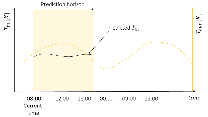
This information can be passed to the MPC to improve the control performance. Let’s see how to do it. First, you need to tell HILO-MPC which of the model parameters are time varying:

nmpc.set_time_varying_parameters(names=['T_out'], values=temp_prediction)

Where T_out is the name of one of the model parameters. The values parameter is a dictionary. This must contain as keys the names of the time-varying parameters and and as values the value of the parameters.

temp_prediction['T_out'] = [21.3, 20.4, ..., 19.4,... 22.4]

Note

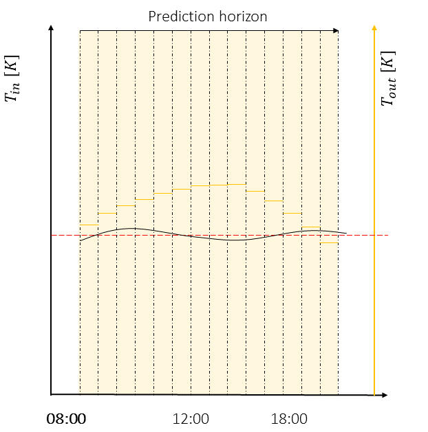
The values must be sampled with the same sampling time of the MPC and they are assumed constant within the sampling time as represented in the following picture

Warning

At the moment the time-varying parameters work only with discrete objective function. Remember to pass 'objective_function'='discrete' to the MPC options if you system is continuous time.

Note

If the supplied value are not covering the entire simulation time plus the prediction horizon, HILO-MPC will automatically repeat the values starting from the beginning. This is useful if you have a periodic time-varying parameter, since in this case you can give only the value of a period.

You can pass the dictionary with the values either in set_time_varying_parameters or directly to the parameter tvp in the optimize method. This allows you, if necessary, to change the values of the parameters directly in the control loop.

Trajectory tracking problem¶

The trajectory tracking problem can be formulated easily. Refer to theoretical background for the theoretical background and to the following examples:

point mass

There are two ways to define a trajectory tracking problem. If you have a time varying function that describes the time-varying reference you can pass it directly to the problem. If instead you have only the values of the references but not the function you can pass the data directly.

Available reference function¶

If the function is available proceed as follows:

Run create_time_variable() to generate the time variable
Define the time-varying function using the time variable
Pass the time function function to the ref argument of stage and terminal cost and put trajectory_tracking=True

for example:

nmpc = NMPC(model)

time = nmpc.create_time_variable()

nmpc.quad_stage_cost.add_states(names=['x', 'y'], weights=[10, 10],
                                ref=[ca.sin(time), ca.sin(2 * time)],
                                trajectory_tracking=True)

nmpc.quad_terminal_cost.add_states(names=['x', 'y'], weights=[10, 10],
                               ref=[ca.sin(time), ca.sin(2 * time)],
                               trajectory_tracking=True)

Note

This works even your system is discrete-time. The toolbox will automatically evaluate the function at the discretization points.

Only values of the references are available¶

Alternatively, you can pass the values directly in this case you need to just put the flag trajectory_tracking=True as follows:

nmpc = NMPC(model)


nmpc.quad_stage_cost.add_states(names=['x', 'y'], weights=[10, 10],
                                trajectory_tracking=True)

nmpc.quad_terminal_cost.add_states(names=['x', 'y'], weights=[10, 10],
                               trajectory_tracking=True)

then you need to pass a matrix of the reference to the optimize method. For example

for step in range(n_steps):
    u = nmpc.optimize(x0, ref_sc=ref_sc_dict,
                      ref_tc=ref_tc_dict)

where ref_sc_dict and ref_tc_dict contain the trajectory that is tracked in the stage cost and in the terminal cost. These are dictionaries where the keys are the names of the variables that have a varying trajectory. In this case x and y and the values are lists that contain the reference for every time point. In this case the objective function must be set to discrete. If the length of the lists is greater than the simulation time plus the horizon length, HILO-MPC will substitue the correct value of the reference at the correct time point. If you pass a scalar, or a list of length one, HILO-MPC will assume that the reference is constant for the entire prediction horizon. This can be usefull for step-wise change in references. For example the code

nmpc = NMPC(model)

nmpc.quad_stage_cost.add_states(names=['x', 'y'], weights=[10, 10], trajectory_tracking=True)
nmpc.quad_terminal_cost.add_states(names=['x', 'y'], weights=[10, 10], trajectory_tracking=True)

nmpc.horizon = 10
nmpc.set_initial_guess(x_guess=x0, u_guess=u0)
nmpc.setup(options={'objective_function': 'discrete'})

model.set_initial_conditions(x0=x0)

ss = SimpleControlLoop(model,nmpc)
ss.run(100, ref_sc={'x':1,'y':2},
       ref_tc={'x':1,'y':2})

ss.run(100, ref_sc={'x':2,'y':1},
       ref_tc={'x':2,'y':1})

runs the system model for 100 steps with references 2 and 1, and successively 100 steps with references 1 and 2for x and y respectively.

Path following problem¶

HILO-MPC allows you do quickly define path-following problems. Here we go into the details of what you can do to setup a path-following problem. For a background on path-following MPC refer to our theoretical background and to our examples:

Note

The fastest way to build a path following problem is using the quadratic cost class hilo_mpc.util.optimizer.QuadraticCost. You can do it also with the generic cost if you really need it, but it will be more involved. For now, we use the QuadraticCost, since it covers 99.9% of the problems you might want to solve (we hope).

Defining a path-following problem can be done in three steps:

Run hilo_mpc.NMPC.create_path_variable() to generate the path variable
Define the path function using the path variable
Pass the path function function to the ref argument of stage and terminal cost and put path_following=True

Note

You can create only as many path variables and you can have as many different path functions as you want.

You can pass to the hilo_mpc.NMPC.create_path_variable():

The name of the variable.
The lower and upper bound on the virtual input.
A constant reference, the virtual input should follow (optional).
The weight on the difference between the reference and value of the virtual input (optional).

here is an example

nmpc = NMPC(model)

# 1. Create the path variable
theta = nmpc.create_path_variable(name='theta', u_pf_ub=0.01, u_pf_lb=0.001,
                                    u_pf_ref=0.04, u_pf_weight=10)

# 2. Define path function using path variable
path = ca.vertcat(ca.sin(theta), ca.sin(2 * theta))

# 3. Tell HILO-MPC that the variables 'x' and 'y' must follow a path following problem by setting
# `path_following` = True
nmpc.quad_stage_cost.add_states(names=['x', 'y'], weights=[10, 10],
                                ref=, path_following=True)

not that in the example we gave a u_pf_ref parameter. Because of that HILO-MPC will automatically add an extra cost to the quadratic stage cost

\[10(u_{\text{pf}} - 0.04)^2\]

such that the virtual input stays as close as possible to the refernece.

Note

You can define the path function with any other variable that appears in the model!

You can also have multiple path variables. To do that just simply call the hilo_mpc.NMPC.create_path_variable() as many times you want. For example

nmpc = NMPC(model)

theta1 = nmpc.create_path_variable(name='theta1', vel_ub=0.01)

nmpc.quad_stage_cost.add_states(names=['x', 'y'], weights=[10, 10],
                                ref=ca.vertcat(ca.sin(theta1), ca.sin(2 * theta1)),
                                path_following=True)

theta2 = nmpc.create_path_variable(name='theta2', vel_ub=0.01)

nmpc.quad_terminal_cost.add_states(names=['x', 'y'], weights=[10, 10],
                                   ref=ca.vertcat(ca.sin(theta2), ca.sin(2 * theta2)),
                                   path_following=True)

Advanced constraints¶

Unless you are using the single-shooting method for the MPC predictions, HILO-MPC optimizes over the states and inputs at every sampling time [here link to integration methods]. You can create any user defined constraint that use any of the state or inputs at any sampling time. This can be done using the set_custom_constraints_function() method. This takes a Python function an upper and lower bound on the constraint.

The Python function takes three arguments: the entire optimization vector, the indices of the states and inputs at every sampling time.

def custom_const(z, x_ind, u_ind):
    constraint = #some math
    return constraint

Debugging the NMPC¶

Sometimes is useful to visualize the single iterations of the optimizer and the the values of the constraints at every point of the prediction horizon. At the moment, the debugger works with ipopt.

IPOPT debugger (beta)¶

To enter the debugging mode it is enough to pass options={ipopt_debugger:True} when setting up the MPC as follows

mpc.setup(options={'ipopt_debugger': True})

In this case, the mpc object will have a debugger object that can be accessed as mpc.debugger. This contains useful information on the intermediate iterations of the NMPC. A quick way to visualize the results is with the method plot_iterations

u = mpc.optimize(x0=x0)
plant.simulate(u=u)
mpc.plot_iterations(plot_last=True)

Note

At the moment the plot_iteration method works only with bokeh.

To visualize the states, pass plot_states= True. Note that if optimizer performs many iterations, the plots could take quite a while to load.

Stochastic Model Predictive Control (Beta)¶

The stochastic MPC is implemented in the class SMPC. At the moment, the current SMPC formulations are implemented.

Taylor approximation with additive uncertainty¶

This considers discrete-time nonlinear systems of the following form

\[\begin{equation} x_{k+1} = f(x_k,u_k) + B \left(g(x_k,u_k) + w_k\right), \end{equation}\]

where \(g(x_k,u_k)\) is uncertain function and \(w_k \sim \mathcal{N}(\mu_w,\Sigma_w)\) is random distributed noise. In the current implementation, the function \(g(x_k,u_k)\) can be a Gaussian process. The stochastic MPC problem reads

\[\begin{split}\begin{align} &\!\max_{\Pi(x)}&\qquad& \mathbb{E} \left( \sum_{k=0}^{N-1} l(x_k,u_k) + e(x_N)\right),\\ &\text{s.t.}&&x_{k+1}=f(x_k,u_k) + B \left(d(x_k,u_k) + w \right), \\ &&& u_k = \pi(x_k), \quad x_0=x(k), \\ &&& \text{Pr} \left(x_{k+1} \in \mathcal{X}\right)\geq p^x, \\ &&&\text{Pr} \left(u_k \in \mathcal{U}\right) \geq p^u. \end{align}\end{split}\]

The previous problem is infinite dimensional hence in general intractable. Following the similar steps as in [Hewing and Zeilinger, 2017], the problem is reformulated as follows

\[\begin{split}\begin{align} &\!\max_{\mu^u}&\,\ & \mathbb{E} \left( \sum_{k=0}^{N-1} l(x_k,u_k) + e(x_N)\right) \\ &\text{s.t.}&&\mu^x_{k+1}=f(\mu^x_k,\mu^u_k) + B \mu_k^d, \\ &&& \Sigma_{k+1}^x = \left[ \nabla f(\mu_i^x,\mu_i^u), B\right] \Sigma_i \left[ \nabla f(\mu_i^x,\mu_i^u), B\right]^{T}, \\ &&& \mu_{k+1}^x \in \bar{\mathcal{X}}(\Sigma^x_{k+1}), \,\ \mu_k^u \in \bar{\mathcal{U}}(\Sigma^x_k),\\ &&& \mu_0^x =x(k),\,\ \Sigma_{0}^x = \Sigma^x(k), \end{align}\end{split}\]

To see how the SMPC can be used, refer to the example [here put example].

Linear Model Predictive Control¶

The linear model predictive control class solves the following problem

\[\begin{split}\min_{\mathbf{u}} \sum_{i=0}^{N-1} \left( x^T_i Q x_i + u^T_i R u_i \right) + x^T_N P x_N \\ x_{i+1} = Ax_i + Bu_i\, \quad x_0 = \hat{x}(t_0)\\ x_{\text{lb}} \leq x \leq x_{\text{ub}} \\ u_{\text{lb}} \leq u \leq u_{\text{ub}} \\ \forall i \in [1,...,N]\end{split}\]

where \(\mathbf{u} = [u_0^T,u_1^T,...,u_{N-1}^T]\). Note that it uses discrete-time linear systems with box constraints. The problem is reformulated as a quadratic programming problem

\[\begin{split}\min_{\mathbf{z}} \mathbf{z} ^T H \mathbf{z} + q\mathbf{z} + f \\ A_{\text{eq}} \mathbf{z} = b_{\text{eq}} \\ A_{\text{d}} \mathbf{z} \leq b_\text{d}\end{split}\]

where \(\mathbf{z} = [\mathbf{x}^T, \mathbf{u}^T]^T\) and \(\mathbf{x} = [x_0^T,x_1^T,...,x_{N}^T]^T\) using a sparse approach.

Time-varying parameters¶

Time-varying can be defined exactly in the same way of the NMPC (see section).

Solvers¶

To solve the LMPC, the it is possible to use any of the solvers supported by CasADi. The default solver is qpoasis, which is dispatched with CasADi. Other solvers are: gurobi, cplex, OOQP, and SQIC among others. See the CasADi documentation for the complete list of the solver as well as the options for every solver. The solver and its options can be set when calling the setup method of the LMPC. For example:

lmpc = LMPC(model) # initialize the LMPC with a linear time-discrete model
# ...
# here sets its parameters, e.g., horizon length etc
# ...
lmpc.setup(solver='qpoases', solver_options={'sparse':True})

Note

The options can vary depending on the solver used.

[HZ17]

Lukas Hewing and Melanie N. Zeilinger. Cautious model predictive control using gaussian process regression. CoRR, 2017. URL: http://arxiv.org/abs/1705.10702, arXiv:1705.10702.