Learning an MPC controller with a NN

The goal of this example is learning a MPC controller using a artificial neural network.

Introduction

Learning a MPC from simulations and use the learned model for real applications could have several advantages [1]. For example for embedded applications often we need to compute the control action in a very short time, with low computational power and low energy (e.g. embedded applications using batteries). For this for this it is useful to learn the controller offline, that basically approximates the solution of the optimization problem given the measured states. The learned controller can be quickly and efficiently evaluated online in the embedded system, without solving an optimization problem.

The system that is considered in this example is a linear mass-spring-damper system, whose dynamics are given by

\[\begin{split}\begin{align} & \dot{x_1} = x_2 \\ & \dot{x_2} = \frac{1}{m} (u - k x_1 - d x_2) \\ \end{align}\end{split}\]

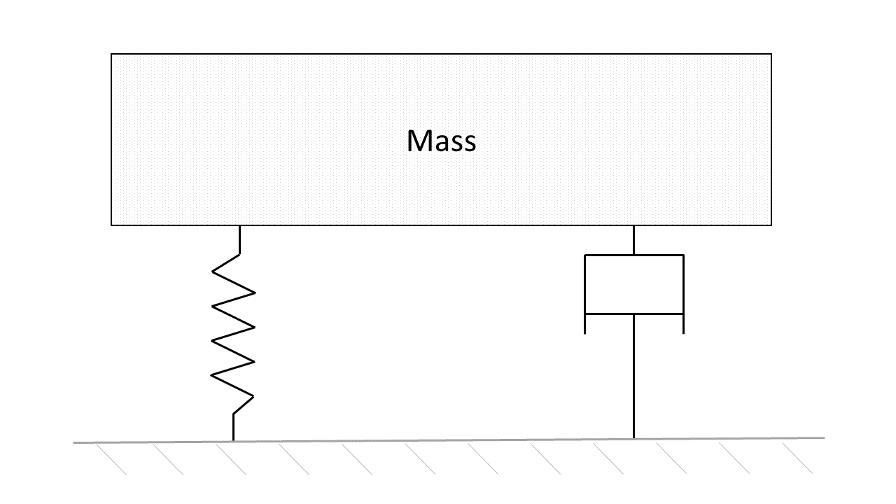
Therein, the state \(x_1\) is the displacement of the mass \(m\), the state \(x_2\) is the velocity of the mass, the input \(u\) is the applied force, \(k\) is the spring constant and \(d\) is the damping factor.

We assume that the states can be measured perfectly, i.e., we will not define a separate output equation.

One sampling period takes \(15~\text{ms}\).

# Add HILO-MPC to path. NOT NECESSARY if it was installed via pip.
import sys
sys.path.append('../../../')

import numpy as np

from hilo_mpc import Model, NMPC, SimpleControlLoop, ANN, Layer

Model

system = Model(plot_backend='bokeh', name='Linear SMD')

# Set states and inputs
system.set_dynamical_states('x', 2)
system.set_inputs('u')

# Add dynamics equations to model
system.set_dynamical_equations(['x_1', 'u - 2 * x_0 - 0.8 * x_1'])

# Sampling time
Ts = 0.015  # Ts = 15 ms

# Set-up
system.setup(dt=Ts)

# Initialize system
x_0 = [12.5, 0]
system.set_initial_conditions(x_0)

Generate data

We start defining the MPC we want to learn as follows.

# Make controller
nmpc = NMPC(system)

# Set horizon
nmpc.horizon = 15

# Set cost function
nmpc.quad_stage_cost.add_states(names=['x_0', 'x_1'], weights=[100, 100], ref=[1, 0])
nmpc.quad_stage_cost.add_inputs(names=['u'], weights=[10], ref=[2])
nmpc.quad_terminal_cost.add_states(names=['x_0', 'x_1'], weights=np.array([[8358.1, 1161.7], [1161.7, 2022.9]]),
                                   ref=[1, 0])
nmpc.set_box_constraints(u_ub=[15], u_lb=[-20])

# Set-up controller
nmpc.setup(options={'print_level': 0})

C:\Users\Bruno\Documents\GitHub\hilo-mpc\hilo_mpc\modules\base.py:2174: UserWarning: Plots are disabled, since no backend was selected.
  warnings.warn("Plots are disabled, since no backend was selected.")

Manuall closed-loop data generation

The data can be generated manually, by running the system as follows

# Vector of simulation time points
Tf = 10  # Final time
t = np.arange(0, Tf, Ts)
n_steps = int(Tf / Ts)
scl = SimpleControlLoop(system, nmpc)
scl.run(n_steps)

scl.plot(output_notebook=True)

Loading BokehJS ...

'C:\\Users\\Bruno\\AppData\\Local\\Programs\\Python\\Python37\\lib\\runpy.py'

Automatic closed-loop data generation

Alternativelly it can be done using the generate_data helper method. We will continue using this method

data_set = system.generate_data('closed_loop', nmpc, steps=n_steps, use_input_as_label=True)
features= data_set.features
labels= data_set.labels

Training

Now we define a NN and train it with the generated dataset.

# Initialize and set up ANN
ann = ANN(features, labels, learning_rate=1e-3)
ann.add_layers(Layer.dense(10, activation='ReLU'))
ann.add_layers(Layer.dense(10, activation='ReLU'))
ann.add_layers(Layer.dense(10, activation='ReLU'))
ann.setup(device='cpu')

# Add dataset
ann.add_data_set(data_set)

# Train NN
ann.train(1, 1000, validation_split=.2, patience=100, verbose=0)

Use the NN in closed loop

We now use the ANN controller instead of the MPC. Note that we start from a different initial conditions from the training data

system.reset_solution(keep_initial_conditions=False)
system.set_initial_conditions(x0=[10, 0])
scl = SimpleControlLoop(system, ann)
scl.run(n_steps)

Plots

# Prepare data for comparison
y_data = []
features, labels = data_set.raw_data
ct = 0
for k, feature in enumerate(data_set.features):
    y_data.append({
        'data': np.append(features[k, :], features[k, -1]),
        'kind': 'line',
        'subplot': ct,
        'label': feature + '_mpc'
    })
    ct += 1
for k, label in enumerate(data_set.labels):
    y_data.append({
        'data': np.append(labels[k, :], labels[k, -1]),
        'kind': 'step',
        'subplot': ct,
        'label': label + '_mpc'
    })
    ct += 1


# Plots
scl.plot(y_data=y_data, output_notebook=True)

Final notes

This is a quick example of an ANN controller hence we did not focus on how to generate a dataset that covers a wide range of states, nor we postprocessed/optimize the datapoints.

.. footbibliography::