Formula 1

In this example we will consider a path-following problem in the presence of an obstacle. In this example we will se how

1. to add hard generic stage and terminal constraints to the MPC.

2. to add soft generic stage and terminal constraints to the MPC.

Introduction

We consider the problem of a racing F1 car along a ellipsoidal track. At some point of the track an obstacle is present due to an accident. For the car model we use a simple bicycle model:

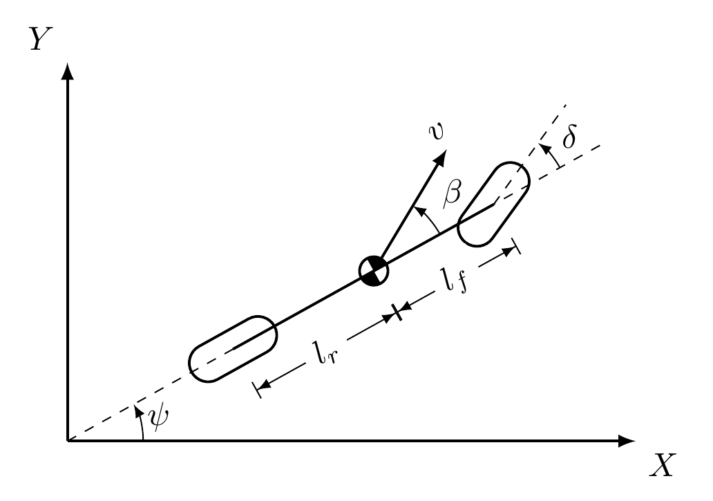
the model equation look like:

\[\begin{split}\begin{align} \dot{p}_X &= v \cos (\psi + \beta), \\ \dot{p}_Y &= v \sin (\psi + \beta), \\ \dot{v} &= a, \\ \dot{\psi} &= \frac{v}{l_r} \sin({\beta}), \\ \beta &= \tan^{-1}\Big(\frac{l_r}{l_f + l_r} \tan({\delta})\Big), \end{align}\end{split}\]

The orientation of the vehicle is denoted by ψ. The control inputs of the model are acceleration a and steering angle δ. The algebraic factor β is known as the slip angle and it represents the angle of motion of the vehicle CoG with respect to the vehicle orientation. The path to follow is an allipse with the following parametric equation:

\[F(\theta) = [\tau_X(\theta), \tau_Y(\theta)] = [30 - 14 \cos(\theta), \,\ 30 - 16 \sin(\theta)]\]

the objective function looks like

\[L = \sum_{i=1}^N \left [(p_{X,i}- \tau_X(\theta_i)) + (p_{Y,i}- \tau_Y(\theta_i)) \right] + (p_{X,{N+1}}- \tau_X(\theta_{N+1})) + (p_{Y,{N+1}}- \tau_Y(\theta_{N+1}))\]

where \(\theta\) is the path variable.

The obstacle is circular with radious \(r=2\) centered in \((obs_{X}, obs_{Y}) = (30, 15)\) will be modelled by adding the following nonlinear constraints

\[c(p_X,p_Y) = (p_X - obs_X)^2 + (p_Y - obs_Y)^2 \geq r^2\]

Simulation

we start importing the necessary modules

# Add HILO-MPC to path. NOT NECESSARY if it was installed via pip.
import sys
sys.path.append('../../../')

from hilo_mpc import Model, NMPC
import casadi as ca
import pandas as pd
import numpy as np

# Necessary for plots
import yaml
from bokeh.layouts import column, layout, row
from bokeh.models import ColumnDataSource, Slider, ImageURL, Band
from bokeh.plotting import figure
from bokeh.themes import Theme
from bokeh.io import show, output_notebook
from bokeh.sampledata.sea_surface_temperature import sea_surface_temperature

output_notebook()

Loading BokehJS ...

Model

model = Model(plot_backend='bokeh')

states = model.set_dynamical_states(['px', 'py', 'v', 'phi'])
inputs = model.set_inputs(['a', 'delta'])

# Unwrap states
px = states[0]
py = states[1]
v = states[2]
phi = states[3]

# Unwrap states
a = inputs[0]
delta = inputs[1]

# Parameters
lr = 1.4  # [m]
lf = 1.8  # [m]
beta = ca.arctan(lr / (lr + lf) * ca.tan(delta))

# ODE
dpx = v * ca.cos(phi + beta)
dpy = v * ca.sin(phi + beta)
dv = a
dphi = v / lr * ca.sin(beta)


model.set_dynamical_equations([dpx, dpy, dv, dphi])

# Initial conditions
x0 = [15, 30, 0, 0]
u0 = [0., 0.]

# Create model and run simulation
dt = 1
model.setup(dt=dt)
model.set_initial_conditions(x0=x0)

Obstacle

We define a round obstacle with radius of 2 meters occupying almost the entire road cross-section.

# Obstacle position and geometry
obs_x = 30
obs_y = 15
obs_rad = 2 #[m]

Setup the MPC

# Setup NMPC
nmpc = NMPC(model)


theta = nmpc.create_path_variable(u_pf_lb=0.1, u_pf_ub=1)

# You can also put the reference on the virtual input
# theta = nmpc.create_path_variable(u_pf_lb=0.1, u_pf_ub=1, u_pf_ref=None, u_pf_weight=10)

path_x = 30 - 14 * ca.cos(theta)
path_y = 30 - 16 * ca.sin(theta)

nmpc.horizon = 30
nmpc.quad_stage_cost.add_states(names=['px', 'py'], ref=ca.vertcat(path_x, path_y), weights=[1, 1],
                                path_following=True)


nmpc.quad_terminal_cost.add_states(names=['px', 'py'], ref=ca.vertcat(path_x, path_y), weights=[1, 1],
                                   path_following=True)

nmpc.set_box_constraints(x_lb=[-100, -100, -10, -100], x_ub=[100, 100, 10, 100], u_lb=[-1, -1], u_ub=[1, 1])

Add nonlinear stage and terminal constraints

nmpc.stage_constraint.constraint = (px - obs_x) ** 2 + (py - obs_y) ** 2
nmpc.stage_constraint.ub = ca.inf
nmpc.stage_constraint.lb = obs_rad ** 2
nmpc.stage_constraint.weight = 10


nmpc.terminal_constraint.constraint = (px - obs_x) ** 2 + (py - obs_y) ** 2
nmpc.terminal_constraint.ub = ca.inf
nmpc.terminal_constraint.lb = obs_rad ** 2
nmpc.terminal_constraint.weight = 10

nmpc.set_initial_guess(x_guess=x0, u_guess=[0, 0])
nmpc.setup(options={'print_level':0})

For plotting we need to create a line representing the path

# Create function to plot the path
pp = ca.SX.sym('pp')
path_x = 30 - (14*pp) * ca.cos(theta)
path_y = 30 - (16*pp) * ca.sin(theta)

path_fun = ca.Function('path',[theta, pp],[path_x,path_y])

x_path = []
y_path = []
for t in range(800):
    x_p, y_p = path_fun(t / 100, 1)
    x_path.append(float(x_p))
    y_path.append(float(y_p))

Simulation

n_steps = 100
for i in range(n_steps):
    u = nmpc.optimize(x0)
    model.simulate(u=u)
    x0 = model.solution['x:f']

******************************************************************************
This program contains Ipopt, a library for large-scale nonlinear optimization.
 Ipopt is released as open source code under the Eclipse Public License (EPL).
         For more information visit http://projects.coin-or.org/Ipopt
******************************************************************************

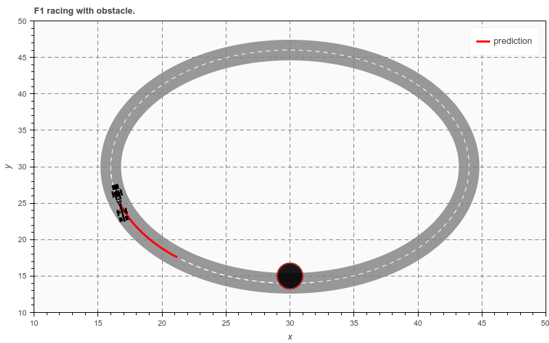
Results

plot = figure(y_range=(10, 50), x_range=(10, 50), y_axis_label='y', x_axis_label='x', title="F1 racing with obstacle.")

plot.line(x=x_path, y=y_path, alpha=0.8, color='grey', line_width=80)
plot.line(x=x_path, y=y_path, line_dash='dashed', color='white')

plot.line(x=np.array(model.solution['px']).squeeze(), y=np.array(model.solution['py']).squeeze(), color='red',
          line_width=3, legend_label='position')
r = plot.circle(x=obs_x, y=obs_y)
glyph = r.glyph
glyph.radius = obs_rad / 2
glyph.fill_alpha = 0.9
glyph.fill_color = 'black'
glyph.line_color = "firebrick"
glyph.line_width = 2

show(plot)

Soft constraints

model.reset_solution()
model.setup(dt=dt)
# Initial conditions
x0 = [15, 30, 0, 0]
model.set_initial_conditions(x0=x0)

# Setup NMPC
nmpc = NMPC(model)


theta = nmpc.create_path_variable(u_pf_lb=0.1, u_pf_ub=1)
path_x = 30 - 14 * ca.cos(theta)
path_y = 30 - 16 * ca.sin(theta)

nmpc.horizon = 30
nmpc.quad_stage_cost.add_states(names=['px', 'py'], ref=ca.vertcat(path_x, path_y), weights=[1, 1], path_following=True)
nmpc.quad_terminal_cost.add_states(names=['px', 'py'], ref=ca.vertcat(path_x, path_y), weights=[1, 1], path_following=True)
nmpc.set_box_constraints(x_lb=[-100, -100, -10, -100], x_ub=[100, 100, 10, 100], u_lb=[-1, -1], u_ub=[1, 1])

nmpc.stage_constraint.constraint = (px - obs_x) ** 2 + (py - obs_y) ** 2
nmpc.stage_constraint.ub = ca.inf
nmpc.stage_constraint.lb = obs_rad ** 2
nmpc.stage_constraint.is_soft =True
nmpc.stage_constraint.max_violation = 0.5

nmpc.terminal_constraint.constraint = (px - obs_x) ** 2 + (py - obs_y) ** 2
nmpc.terminal_constraint.ub = ca.inf
nmpc.terminal_constraint.lb = obs_rad ** 2
nmpc.terminal_constraint.is_soft = True
nmpc.terminal_constraint.max_violation = 0.5

nmpc.set_initial_guess(x_guess=x0, u_guess=[0, 0])
nmpc.setup(options={'print_level':0})

for i in range(n_steps):
    u = nmpc.optimize(x0)
    model.simulate(u=u)
    x0 = model.solution['x:f']

Results

plot = figure(y_range=(10, 50), x_range=(10, 50), y_axis_label='y', x_axis_label='x', title="F1 racing with obstacl.")

plot.line(x=x_path, y=y_path, alpha=0.8, color='grey', line_width=80)
plot.line(x=x_path, y=y_path, line_dash='dashed', color='white')

plot.line(x=np.array(model.solution['px']).squeeze(), y=np.array(model.solution['py']).squeeze(), color='red',
          line_width=3, legend_label='position')
r = plot.circle(x=obs_x, y=obs_y)
glyph = r.glyph
glyph.radius = obs_rad / 2
glyph.fill_alpha = 0.9
glyph.fill_color = 'black'
glyph.line_color = "firebrick"
glyph.line_width = 2

show(plot)