Path following vs Trajectory Tracking MPC

Introduction

In this example we will see how to define trajectory tracking and path following control problems using Neo.

For this example we consider a point mass. The goal is to follow this shape by using a path-following approach.

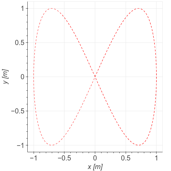
the equation that describe it are \(x(\theta) = sin(\theta)\) and \(y(\theta) = sin(2 \theta)\).

First import the necessary packages

# Add NMPC to path. NOT NECESSARY if it was installed via pip.
import sys
sys.path.append('../../../')

# Import NMPC and Model classes
from hilo_mpc import NMPC, Model
import casadi as ca

Build the model

# Define the model
model = Model(plot_backend='bokeh')

# Constants
M = 5.

# States and algebraic variables
xx = model.set_dynamical_states(['x', 'vx', 'y', 'vy'])
model.set_measurements(['y_x', 'y_vx', 'y_y', 'y_vy'])
model.set_measurement_equations([xx[0], xx[1], xx[2], xx[3]])
x = xx[0]
vx = xx[1]
y = xx[2]
vy = xx[3]

# Inputs
F = model.set_inputs(['Fx', 'Fy'])
Fx = F[0]
Fy = F[1]

# ODEs
dd1 = vx
dd2 = Fx / M
dd3 = vy
dd4 = Fy / M

model.set_dynamical_equations([dd1, dd2, dd3, dd4])

# Initial conditions
x0 = [0, 0, 0, 0]
u0 = [0., 0.]

# time interval
dt = 0.1
model.setup(dt=dt)

Path-following problem

Once the model is setup, we can pass it to the path-following MPC. Defining a path-following problem can be done in 3 steps:

1. Run create_path_variable() to generate the path variable

2. Define the path function using the path variable

3. Pass the path function function to the ref argument of stage and terminal cost and put path_following=True

NOTE: you can create only as many path variables and you can have as many different path functions as you want.

# Define path following MPC
nmpc = NMPC(model)
theta = nmpc.create_path_variable(u_pf_lb=1e-6)
nmpc.quad_stage_cost.add_states(names=['x', 'y'], weights=[10, 10],
                                ref=ca.vertcat(ca.sin(theta), ca.sin(2 * theta)), path_following=True)
nmpc.quad_terminal_cost.add_states(names=['x', 'y'], weights=[10, 10],
                                   ref=ca.vertcat(ca.sin(theta), ca.sin(2 * theta)), path_following=True)
nmpc.horizon = 10
nmpc.set_initial_guess(x_guess=x0, u_guess=u0)
nmpc.setup(options={'print_level': 0})

Then run the control loop

# Prepare and run closed loop
n_steps = 200
model.set_initial_conditions(x0=x0)
sol = model.solution
xt = x0.copy()
for step in range(n_steps):
    u = nmpc.optimize(xt)
    model.simulate(u=u)
    xt = sol['x:f']

******************************************************************************
This program contains Ipopt, a library for large-scale nonlinear optimization.
 Ipopt is released as open source code under the Eclipse Public License (EPL).
         For more information visit http://projects.coin-or.org/Ipopt
******************************************************************************

The results look like

from bokeh.io import output_notebook, show
from bokeh.plotting import figure, gridplot
import numpy as np

# define path function for plotting
def path(theta):
    return np.sin(theta), np.sin(2 * theta)
x_path = []
y_path = []
for t in range(1000):
    x_p, y_p = path(t / 100)
    x_path.append(x_p)
    y_path.append(y_p)

# Plot using bokeh
output_notebook()
p_pf = figure(title='Path following problem')
p_pf.line(x=np.array(model.solution['x']).squeeze(), y=np.array(model.solution['y']).squeeze())
p_pf.line(x=x_path, y=y_path, line_color='red', line_dash='dashed')
# p = format_figure(p)
p_pf.yaxis.axis_label = "y [m]"
p_pf.xaxis.axis_label = "x [m]"
show(p_pf)

Loading BokehJS ...

Trajectory tracking problem

Trajectory tracking problems are formulated similarly to path following problem. For the case where the function of the trajectory is available, do as follows:

1. Run create_time_variable() to generate the time variable

2. Define the time-varying function using the time variable

3. Pass the time function function to the ref argument of stage and terminal cost and put trajectory_tracking=True

NOTE: if the function of the reference is not available, you can pass directly the data points when solving the MPC. see the documentation for more info.

# Define trajectory tracking MPC
nmpc = NMPC(model)
time = nmpc.get_time_variable()
nmpc.quad_stage_cost.add_states(names=['x', 'y'], weights=[10, 10],
                                ref=ca.vertcat(ca.sin(time), ca.sin(2 * time)), trajectory_tracking=True)
nmpc.quad_terminal_cost.add_states(names=['x', 'y'], weights=[10, 10],
                                   ref=ca.vertcat(ca.sin(time), ca.sin(2 * time)), trajectory_tracking=True)
nmpc.horizon = 10
nmpc.set_initial_guess(x_guess=x0, u_guess=u0)
nmpc.setup(options={'print_level': 0})

The rest is the same

# Prepare and run closed loop
n_steps = 100
# the solution stored in the model must be reset (initial conditions are kept by default)
model.reset_solution()
sol = model.solution
xt = x0.copy()
for step in range(n_steps):
    u = nmpc.optimize(xt)
    model.simulate(u=u)
    xt = sol['x:f']

x_path = []
y_path = []
for t in range(1000):
    x_p, y_p = path(t / 100)
    x_path.append(x_p)
    y_path.append(y_p)

# plot using bokeh
output_notebook()
p_tt = figure(title='Trajectory tracking problem')
p_tt.line(x=np.array(model.solution['x']).squeeze(), y=np.array(model.solution['y']).squeeze())
p_tt.line(x=x_path, y=y_path, line_color='red', line_dash='dashed')
# p = format_figure(p)
p_tt.yaxis.axis_label = "y [m]"
p_tt.xaxis.axis_label = "x [m]"
show(p_tt)

Loading BokehJS ...

Comparison

from bokeh.models import Range1d

p_pf.x_range = Range1d(-1,-0.5)
p_pf.y_range = Range1d(0.5, 1)

p_tt.x_range = Range1d(-1,-0.5)
p_tt.y_range = Range1d(0.5, 1)

show(gridplot([p_pf,p_tt], ncols=2))