Inverted pendulum - DAE System¶

Introduction¶

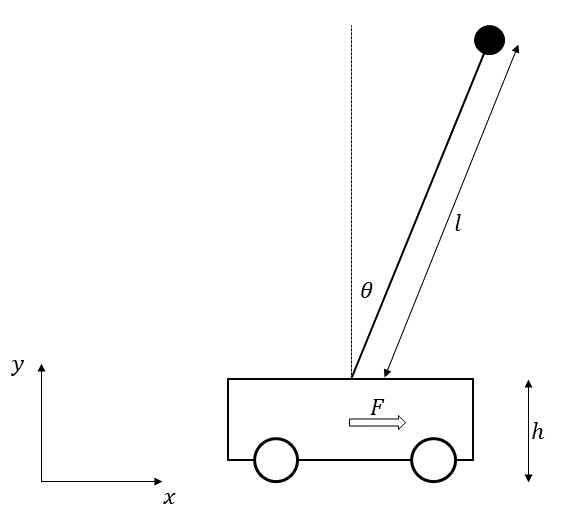
This example shows the simulation and control of an inverted pendulum on a cart. We are going to use this example to show how your can add algebraic equations to the model

The differential algebraic system of the inverted pendulum is given by the following equations:

Model¶

\[\begin{split}\begin{align} \dot{x} &= v \\ \dot{v} &= \frac{(3/4mg\sin(\theta)\cos(\theta) - 1/2ml\sin(\theta)\omega^2 + F)}{(M + m - 3/4m\cos(\theta)^2)} \\ \dot{\theta} &= \omega\\ \dot{\omega} &= \frac{3}{(2l)} (\dot{v}\cos(\theta) + g\sin(\theta))\\ y =& h + l\cos(theta) \end{align}\end{split}\]

The differential and algebraic states are:

\(x\): x-Position of the mass M [m]
\(v\): Linear velocity of the mass M [m/s]
\(\theta\): Angle of the metal rod [rad]
\(\omega\): Angular velocity of the mass m [rad/s]
\(y\): y-Position of the mass M [m]

The inputs that could be applied to control the system are:

\(F\): Force applied to the cart [kg*m/s^2]

The constants of the system are:

\(M\): Mass of the cart [kg]
\(m\): Mass of the pendulum [kg]
\(l\): Length of the lever arm [m]
\(h\): Height of the rod connection [m]
\(g\): Gravitational acceleration [m/s^2]

Objective¶

The objective is to stabilize the weight attached to the rod at \(\theta = 0\) and keep the cart still i.e. \(v=0\). The control problem is the following:

\[\begin{split}\begin{align} &\!\max_{\mathbf{u}(\cdot)}&\qquad& \sum_{i=1}^{N}10 v(t_i)^2 + 5 \theta(t_i)^2 + 0.1F(t_i)^2 + 10v(t_{N+1})^2 + 5\theta(t_{N+1})^2 \\ &\text{s.t.}&&\dot{x}=f(x,u),\quad x(0)=x_0\\ &&&x \in [x_{lb}, x_{ub}], \,\ u \in [u_{lb}, u_{ub}]. \end{align}\end{split}\]

Modelling with Neo¶

Neo can solve use model containing differential algebraic equations (DAEs). These can be added created in three steps:

Create the algebraic variables with the set_algebraic_variables method
Use the algebraic variables in the model.
Add the algebraic equations using the set_algebraic_equations method. Note that the algebraic equations must be in the form \(g(x,z)=0\)

Remember to give an initial guess for the algebraic variable.

[1]:

# Add HILO-MPC to path. NOT NECESSARY if it was installed via pip.
import sys
sys.path.append('../../../')

from hilo_mpc import NMPC, Model
import casadi as ca

import warnings
warnings.filterwarnings("ignore")

model = Model(plot_backend='bokeh')

# Constants
M = 5.
m = 1.
l = 1.
h = .5
g = 9.81

# States and algebraic variables
x = model.set_dynamical_states(['x', 'v', 'theta', 'omega'])
model.set_measurements(['yx', 'yv', 'ytheta', 'tomega'])
model.set_measurement_equations([x[0], x[1], x[2], x[3]])
y = model.set_algebraic_states(['y'])

# Unwrap states
v = x[1]
theta = x[2]
omega = x[3]

# Define inputs
F = model.set_inputs('F')

# ODEs
dd = ca.SX.sym('dd', 4)
dd[0] = v
dd[1] = 1. / (M + m - m * ca.cos(theta)) * (m * g * ca.sin(theta) - m * l * ca.sin(theta) * omega ** 2 + F)
dd[2] = omega
dd[3] = 1. / l * (dd[1] * ca.cos(theta) + g * ca.sin(theta))


# Algebraic equations (note that it is written in the form rhs = 0)
rhs = h + l * ca.cos(theta) - y

# Add differential equations
model.set_dynamical_equations(dd)

# Add algebraic equations
model.set_algebraic_equations(rhs)

# Initial conditions
x0 = [2.5, 0., 0.1, 0.]


# Initial guess algebraic states
z0 = h + l * ca.cos(x0[2]) - h
#Initial guess input
u0 = 0.

# Setup the model
dt = .1
model.setup(dt=dt)

Solver 'cvodes' is not suitable for DAE systems. Switching to 'idas'...

Alternativelly you can define the model more compactly in string form. HILO-MPC will parse it for you

[2]:

# model = Model(plot_backend='bokeh')

# # Define system
# equations = """
# # Constants
# M = 5
# m = 1
# l = 1
# h = 0.5
# g = 9.81

# # DAE
# dx(t)/dt = v(t)
# dv(t)/dt = 1/(M + m - 3/4*m*cos(theta(t))^2) * (3/4*m*g*sin(theta(t))*cos(theta(t)) ...
# - 1/2*m*l*sin(theta(t))*omega(t)^2 + F(k))
# d/dt(theta(t)) = omega(t)
# d/dt(omega(t)) = 3/(2*l) * (dv(t)/dt*cos(theta(t)) + g*sin(theta(t)))
# 0 = h + l*cos(theta(t)) - y(t)
# """
# model.set_equations(equations)

# # Setup model
# model.setup(dt=dt)

NMPC with Neo¶

[3]:

nmpc = NMPC(model)

nmpc.quad_stage_cost.add_states(names=['v', 'theta'], ref=[0, 0], weights=[10, 5])

nmpc.quad_stage_cost.add_inputs(names='F', weights=0.1)

nmpc.horizon = 25

nmpc.set_box_constraints(x_ub=[5, 10, 10, 10], x_lb=[-5, -10, -10, -10])

nmpc.set_initial_guess(x_guess=x0, u_guess=u0)

nmpc.setup(options={'print_level': 0})

n_steps = 100

model.set_initial_conditions(x0=x0, z0=z0)

sol = model.solution

for step in range(n_steps):
    u = nmpc.optimize(x0)
    model.simulate(u=u, steps=1)
    x0 = sol['x:f']


******************************************************************************
This program contains Ipopt, a library for large-scale nonlinear optimization.
 Ipopt is released as open source code under the Eclipse Public License (EPL).
         For more information visit http://projects.coin-or.org/Ipopt
******************************************************************************

Plots¶

Here the results. The plotting will be automatize such that you can quickly get the plots without writing much.

[5]:

from bokeh.io import output_notebook, show
from bokeh.plotting import figure
from bokeh.layouts import gridplot
import numpy as np

output_notebook()
p_tot = []
for state in model.dynamical_state_names:
    p = figure(background_fill_color="#fafafa", width=300, height=300)
    p.line(x=np.array(sol['t']).squeeze(), y=np.array(sol[state]).squeeze(),
           legend_label=state, line_width=2)
    for i in range(len(nmpc.quad_stage_cost._references_list)):
        if state in nmpc.quad_stage_cost._references_list[i]['names']:
            position = nmpc.quad_stage_cost._references_list[i]['names'].index(state)
            value = nmpc.quad_stage_cost._references_list[i]['ref'][position]
            p.line([np.array(sol['t'][1]).squeeze(), np.array(sol['t'][-1]).squeeze()],
                   [value, value], legend_label=state + '_ref',
                   line_dash='dashed', line_color="red", line_width=2)

    p.yaxis.axis_label = state
    p.xaxis.axis_label = 'time'
    p.yaxis.axis_label_text_font_size = "12pt"
    p.yaxis.major_label_text_font_size = "12pt"
    p.xaxis.major_label_text_font_size = "12pt"
    p.xaxis.axis_label_text_font_size = "12pt"

    p_tot.append(p)

show(gridplot(p_tot, ncols=2))

Loading BokehJS ...